Chapter 6 Modeling
For our first pass a submission, we are going to use the XGBoost model. This model has seen much success in Kaggle competitions and wide use across industry and academia due to its flexiblity, speed, and range of modeling tasks it can be applied to. We’ll start by creating a base line model and then try our hand at tuning a few of the XGBoost parameters to see how of performance changes.
6.1 XGBoost
XGBoost, which stands for eXtreme Gradient Boosting, is a highly optimized and flexible implementation of gradient boosted decision trees. At a high level boosted trees work by creating ensembles of decision trees and uses gradient boosting (additive training) to combine each of the tree’s predictions into one strong prediction by optimizing over any differentiable loss function. In practice a regularization penalty is added to the loss function to help control complexity.
Decision trees, particularly XGBoost is widely used for several reasons such as its flexibilty to be used for numerous problem types across both regression and classification, it’s invariance to scaling inputs, and it’s ability to scale to handle large amounts of data.
For more information about XGBoost see Chen & Guestrin1 and Gradient Boosting in general, Fridmean (1999)2
6.2 Our Recipe for Success
As a reminder our recipe for our transformations are stored in rec that we created in Chapter 4. It’s looks like this
rec## Data Recipe
##
## Inputs:
##
## role #variables
## outcome 1
## predictor 98
##
## Operations:
##
## Mean Imputation for starts_with("roll_")
## Zero variance filter on all_numeric()
## Box-Cox transformation on 6 items
## Dummy variables from all_nominal()
## Interactions with starts_with("tax_"):starts_with("area_")
## Centering for all_numeric(), -all_outcomes()
## Scaling for all_numeric(), -all_outcomes()
## PCA extraction with starts_with("acs_home_value_cnt")
## Zero variance filter on all_numeric()6.3 Base Line Model
Alice: “Would you tell me, please, which way I ought to go from here?”
The Cheshire Cat: “That depends a good deal on where you want to get to.”
Alice: “I don’t much care where.”
The Cheshire Cat: “Then it doesn’t matter which way you go.”
— The Adventures of Alice in Wonderland, on the need for base line models in machine learning (that’s my interpretation at least)
Making Predictive models is an iterative process, a process in which it is easy to get pulled in wrong directions by needless complexity, fruitless tweaks, and soul crushingly poor performing ideas you thought might actually work.
To help tether ourselves to reality, it is useful to generate a base line model to compare all other models against before we get into any of the more complex tasks like parameter tuning. This will help guide what direction we should take next so we don’t end up like Alice.
Kaggle competitions have done wonders for our collective obession for improving predictive accuracy with wild disregard for the time and effort it took to achieve that improvement. In a typical business or scientific academic application, improvement in predictive accuracy has to be balanced with the cost of acheiving it. A base line model can help use measure these diminishing returns.
For our base line model, we will use the top 20 features returned from our feature selection process in an xgboost model with default parameter settings and with nrounds, the maximum number of boosting iterations, set to 1000
features_to_use_baseline <- feature_avg %>%
  arrange(desc(mean)) %>%
  head(20) %>%
  .$Feature

d_prepped <- prep(rec)

train_df <- bake(d_prepped, newdata = d)

x_train <- train_df %>%
  select(features_to_use_baseline) %>%
  as.matrix()

y_train <- train_df$log_error

xgb_train_data <- xgb.DMatrix(x_train, label = y_train)

base_model <- xgb.train(data = xgb_train_data,
                        objective = 'reg:linear',
                        verbose = FALSE,
                        nrounds = 1000,
                        nthread = 20)
6.3.1 Making Predictions with Base Line Model
Now we finally get to make our first predictions! Since we’ll be doing this again and potentially many times, let’s make a helper function predict_date() to do this. This function will take, the parcels (parcel_id) and the dates (predict_date) we wish to predict, along with the model (mdl) and features we want to use to (features_to_use) to do the predictions
predict_date <- function(parcel_id, predict_date, mdl, features_to_use) {

d_predict_ids <- properties %>%
  filter(id_parcel %in% parcel_id) %>%
  crossing(date = predict_date)

d_predict <- d_predict_ids %>%
  mutate(
    year = year(date),
    month_year = make_date(year(date), month(date)),
    month = month(date, label = TRUE),
    week = floor_date(date, unit = "week"),
    week_of_year = week(date),
    week_since_start = (min(date) %--% date %/% dweeks()) + 1,
    wday = wday(date, label = TRUE),
    day_of_month = day(date)
  ) %>%
  left_join(econ_features, by = "date") %>%
  left_join(roll_bg, by = c("id_geo_bg_fips", "date")) %>%
  left_join(roll_tract, by = c("id_geo_tract_fips", "date")) %>%
  select(
    -id_parcel,
    -week,
    -region_city,
    -region_zip,
    -area_lot_jitter,
    -area_lot_quantile,
    -lat, # we have other lat/lon features
    -lon,
    -starts_with("id_geo")
  ) %>%
  mutate(
    date = as.numeric(date),
    year = factor(year, levels = sort(unique(year)), ordered = TRUE),
    month_year = factor(
      as.character(month_year),
      levels = as.character(unique(sort(month_year))),
      ordered = TRUE),
    str_quality = factor(str_quality, levels = 12:1, ordered = TRUE)
  )

eval_df <- bake(d_prepped, newdata = d_predict)

x_eval <- eval_df %>%
  select(features_to_use) %>%
  as.matrix()

preds <- predict(mdl, x_eval)

properties_predict <- d_predict_ids %>%
  select(
    id_parcel,
    date
  ) %>%
  mutate(
    pred = preds
    ) %>%
  spread(date, pred)

names(properties_predict) <- c("ParcelId", "201610", "201611",
                               "201612", "201710", "201711", "201712")

properties_predict

}
The submission requires a prediction for Oct-Dec 2016 and Oct-Dec 2017. This means that the prediction is for any day in that month. For our example submissions, we are going to set the date to the first Wednesday in each month. This is completely arbitrary, but provides a simple starting point. Another approach would be to make predictions for every day in each month and submit the mean prediction for each month. We’ll save this for later work.
# first wednesday in each month
predict_dates <- date(c("2016-10-06", "2016-11-02", "2016-12-07",
                        "2017-10-04", "2017-11-01", "2017-12-06"))

# split parcels to chunck our predictions
id_parcels <- properties$id_parcel
id_parcel_splits <- split(id_parcels, ceiling(seq_along(id_parcels) / 5000))
Now make the predictions with base_model
base_predict_list <- lapply(id_parcel_splits, function(i) {

  pred_df <- predict_date(
    parcel_id = i,
    predict_date = predict_dates,
    mdl = base_model,
    features_to_use = features_to_use_baseline
    )
  })

# they only evaluate to 4 decimcals so round to save space
# Convert ParcelId to integer to prevent Sci Notation that causes
# issues with submission
base_predict_df <- bind_rows(base_predict_list) %>%
  mutate_at(vars(`201610`:`201712`), round, digits = 4) %>%
  mutate(ParcelId = as.integer(ParcelId)) %>%
  as.data.frame()

write_csv(base_predict_df, "submissions/base_submit.csv")
The resulting MAE of this submission was 0.0789722 on the public leaderboard. Not that great, but hey at least we have room to improve.
Save this value for comparison
base_mae <- 0.0789722Let’s see if tuning the parameters of the XGBoost model can help improve that.
6.4 Hyperparameter Optimization
The double edged sword of the XGBoost model is how widely varying the predictions it generates can be depending on what the models hyperparameters are set to. The good is that it allows us to be very flexible across many different datasets, the bad is it almost always requires us to perform some type of hyperparameter optimization to fine tune its’ performance. The ugly is the code needed to perform this.
Our parameter optimization strategy is as follows
Create a scoring function to capture model performance using MAE
Use 5-fold cross validation to resample our training data
Randomly generate intital parameter combinations.
Using step 3 as an intital input, use a surrogate Random Forest model to progressively zoom into parameter space based on the average performance of parameter sets across the resampled data on our scoring function. We will set this to 4 runs for now, zooming further down each time.
6.4.1 Creating Our Scoring Function
To assess our parameter tuning performance we will create the function xgboost_regress_score() that will capture the MAE of each resample and parameter combination of our data
# create scoring function -------------------------------------------------

xgboost_regress_score <- function(train_df, target_var, params, eval_df, ...) {

    X_train <- train_df %>%
      select(features_to_use) %>%
      as.matrix()

    y_train <- train_df[[target_var]]
    xgb_train_data <- xgb.DMatrix(X_train, label = y_train)

    X_eval <- eval_df %>%
      select(features_to_use) %>%
      as.matrix()

    y_eval <- eval_df[[target_var]]

    xgb_eval_data <- xgb.DMatrix(X_eval, label = y_eval)

    model <- xgb.train(params = params,
                       data = xgb_train_data,
                       watchlist = list(train = xgb_train_data, eval = xgb_eval_data),
                       objective = 'reg:linear',
                       verbose = FALSE,
                       nthread = 20,
                       ...)

    preds <- predict(model, xgb_eval_data)

    list(mae = MAE(preds, y_eval))

  }
6.4.2 Parameter Search Space
We will use the following parameters
eta[default=0.3, alias:learning_rate]- Step size shrinkage used in update to prevents overfitting. After each boosting step, we can directly get the weights of new features, and eta shrinks the feature weights to make the boosting process more conservative.
- range: [0, 1]
gamma[default=0, alias:min_split_loss]- Minimum loss reduction required to make a further partition on a leaf node of the tree. The larger
gammais, the more conservative the algorithm will be. - range[0,
Inf]
- Minimum loss reduction required to make a further partition on a leaf node of the tree. The larger
max_depth[default=6]- Maximum depth of a tree. Increasing this value will make the model more complex and more likely to overfit. 0 indicates no limit.
- range: [0,
Inf]
min_child_weight[default=1]- Minimum sum of instance weight (hessian) needed in a child. If the tree partition step results in a leaf node with the sum of instance weight less than
min_child_weight, then the building process will give up further partitioning. In linear regression task, this simply corresponds to minimum number of instances needed to be in each node. The largermin_child_weightis, the more conservative the algorithm will be. - range: [0,
Inf]
- Minimum sum of instance weight (hessian) needed in a child. If the tree partition step results in a leaf node with the sum of instance weight less than
subsample[default=1]- Subsample ratio of the training instances. Setting it to 0.5 means that XGBoost would randomly sample half of the training data prior to growing trees. and this will prevent overfitting. Subsampling will occur once in every boosting iteration.
- range: (0, 1]
colsample_bytree[default=1]- Subsample ratio of columns when constructing each tree. Subsampling will occur once in every boosting iteration.
- range: (0, 1]
Based on the performance of these optimizations other parameters could be included later. I set the ranges on these parameters with the idea that our base line model might be overfiting.
library(ParamHelpers)
# make parameter set ------------------------------------------------------
xgboost_random_params <-
  makeParamSet(
    makeIntegerParam('max_depth', lower = 1, upper = 15),
    makeNumericParam('eta', lower = 0.01, upper = 0.1),
    makeNumericParam('gamma', lower = 0, upper = 5),
    makeIntegerParam('min_child_weight', lower = 1, upper = 100),
    makeNumericParam('subsample', lower = 0.25, upper = 0.9),
    makeNumericParam('colsample_bytree', lower = 0.25, upper = 0.9)
  )
6.4.3 5-fold Cross Validation
Set up our resampling via 5 fold cross validation
# create cv resampling ----------------------------------------------------
resamples <- vfold_cv(d, v = 5)
6.4.4 Random Forest Search of Parameter Space
All of the heavy lifting for the surrogate Random Forest model is contained in the tidytune::surrogate_search() function.
The progressive zoom into more promising parameter space is done by passing a vector to n and n_canidates. Higher values for n_candidates will restrict the search to better performing areas and lower values increase the randnomness (with 0 falling back on random search).n is the number of runs of the surrogate model that will run for each of our 5 folds.
top_n is set to 5, which tells the model out of the top n_candidates pass along the top_n to the next round.
We will do for runs of the surrogate Random Forest model, zooming into more performant parameter space each time.
library(MLmetrics)
library(xgboost)
library(tidytune)

# perform surrogate search over parameters --------------------------------
n <- c(10, 5, 3, 2)
# start with random and then zoom in
n_candidates <- c(0, 10, 100, 1000)

search_results <-
  surrogate_search(
    resamples = resamples,
    recipe = rec,
    param_set = xgboost_random_params,
    n = n,
    scoring_func = xgboost_regress_score,
    nrounds = 1000,
    early_stopping_rounds = 20,
    eval_metric = 'mae',
    input = NULL,
    surrogate_target = 'mae',
    n_candidates = n_candidates,
    top_n = 5
  )
search_summary <-
search_results %>%
group_by_at(getParamIds(xgboost_random_params)) %>%
summarise(mae = mean(mae)) %>%
arrange(mae)6.4.5 Exploring Parameter Space
Let’s explore the parameter space some, shall we?
search_results %>%
   group_by_at(
     c("surrogate_run",
       "surrogate_iteration",
       "param_id",
      getParamIds(xgboost_random_params)
       )
     ) %>%
   summarise(mae = mean(mae)) %>%
   ungroup() %>%
  mutate(surrogate_run = factor(surrogate_run)) %>%
ggplot(aes(x = subsample, y = gamma, size = mae)) +
  geom_point(aes(col = surrogate_run)) +
  theme_bw() +
  labs(
    y = "gamma",
    x = "subsample",
    col = "Surrogate Run",
    size = "Average MAE"
  )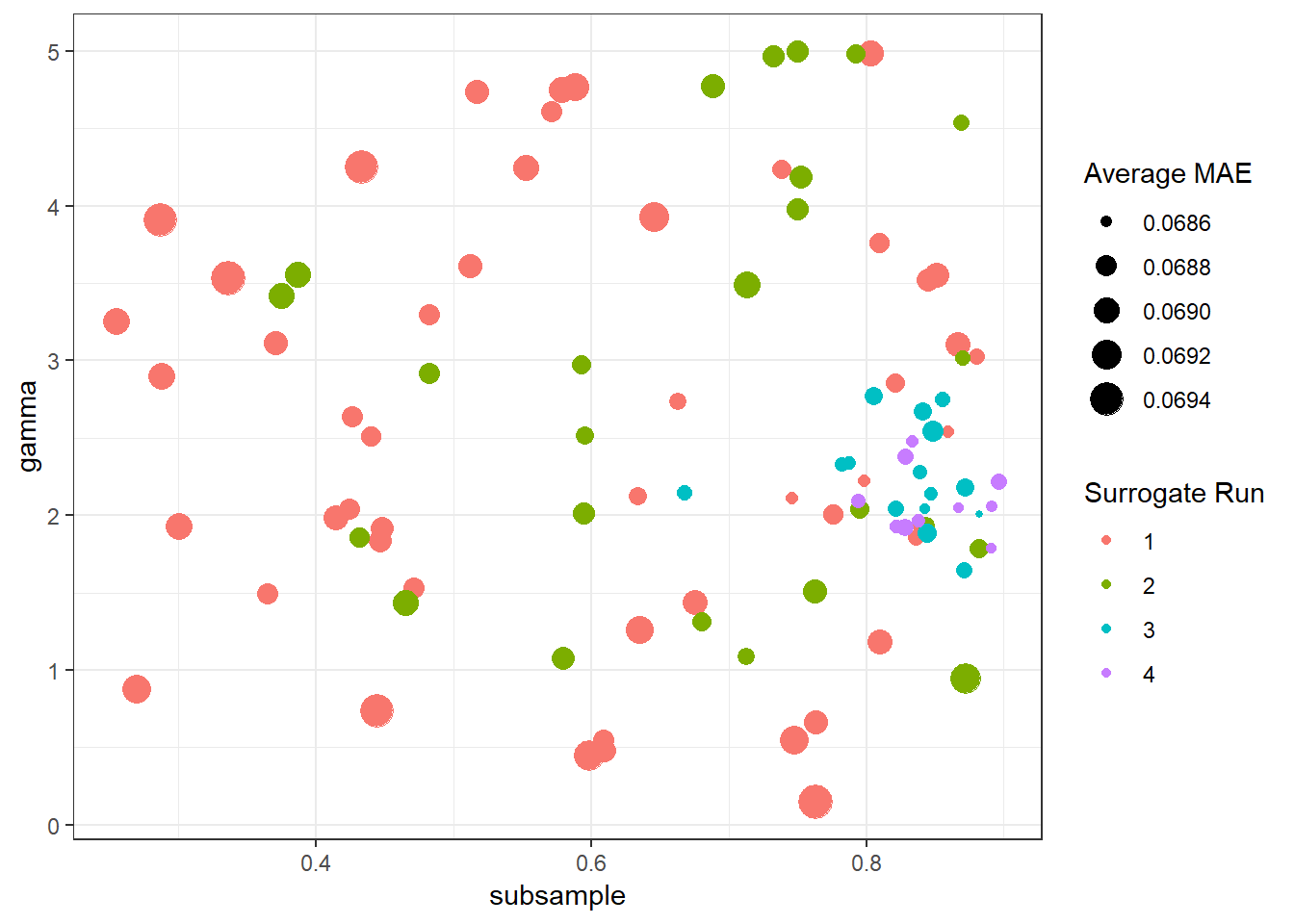
Figure 6.1: Gamma and subsample parameters converging with each surrogate run
How does performance increase with each iteration?
search_results %>%
  group_by_at(
    c("surrogate_run",
      "surrogate_iteration",
      "param_id",
       getParamIds(xgboost_random_params)
      )
    ) %>%
  summarise(mae = mean(mae)) %>%
  ungroup() %>%
  mutate(surrogate_run = factor(surrogate_run)) %>%
  arrange(
    surrogate_run,
    surrogate_iteration
  ) %>%
  mutate(
    iteration = row_number()
  ) %>%
ggplot(aes(x = iteration, y = mae)) +
    geom_smooth(alpha = 0.2, size = 0.8, colour = "grey") +
  geom_point(aes(col = surrogate_run)) +
  theme_bw() +
  labs(
    y = "MAE",
    x = "iteration",
    col = "Surrogate Run"
  )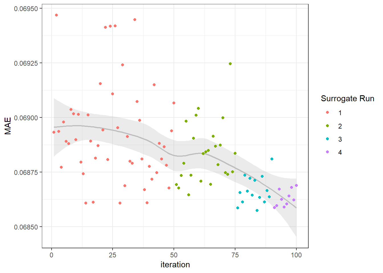
Figure 6.2: Mean Absolute Error Progressively Decreasing with Each Surrogate Run
6.5 Tuned Model
Get the parameter set with the lowest average mae across all folds
tuned_params <- search_summary %>%
  ungroup() %>%
  filter(mae == min(mae)) %>%
  select(getParamIds(xgboost_random_params)) %>%
  as.list()

tuned_params
## $max_depth
## [1] 5
##
## $eta
## [1] 0.07531416
##
## $gamma
## [1] 2.009971
##
## $min_child_weight
## [1] 100
##
## $subsample
## [1] 0.8821157
##
## $colsample_bytree
## [1] 0.5284899Since we didn’t save the actual models produced in our search, train a model with the tuned parameters
d_prepped <- prep(rec)

train_df <- bake(d_prepped, newdata = d)

x_train <- train_df %>%
  select(features_to_use) %>%
  as.matrix()

y_train <- train_df$log_error

xgb_train_data <- xgb.DMatrix(x_train, label = y_train)

tuned_model <- xgb.train(params = tuned_params,
                         data = xgb_train_data,
                         objective = 'reg:linear',
                         verbose = FALSE,
                         nthread = 20,
                         nrounds = 1000)
6.5.1 Making Predictions with Tuned Model
Since we already created our helper function predict_dates() we can apply it here with our new model
predict_list <- lapply(id_parcel_splits, function(i) {

  pred_df <- predict_date(
    parcel_id = i,
    predict_date = predict_dates,
    mdl = tuned_model,
    features_to_use = features_to_use
    )
  })


predict_df <- bind_rows(predict_list) %>%
  mutate_at(vars(`201610`:`201712`), round, digits = 4) %>%
  mutate(ParcelId = as.integer(ParcelId)) %>%
  as.data.frame()

write_csv(predict_df, "submissions/submit01.csv")
6.6 Model Comparison
This model produced a MAE of 0.0651839 on the public leaderboard.
tuned_mae <- 0.0651839

# how much did we improve?
(tuned_mae - base_mae) / base_mae
## [1] -0.1745969Hey not bad! Our hyperparameter optimization process resulted in a 17.5% reduction in Mean Abosolute Error when compared to our base line model. While our absolute position on the leaderboard still isn’t very high, it’s a solid first submission that we can build upon and test new models against. With the top 10 finsishers on the public leaderboard all averaging 184 submissions each (highest being 449!) this empahsizes the iterative nature of predictive modeling. We aren’t in 1st place with our first submission but we didn’t expect to be.
At this point if we were competing the actual competition we would go back to the drawing board in start investigating what we could do differently to improve our score. In our specific case, things like not making the predicion date the first Wednesday of each month and looking at the average prediction across all days in the month would be the first thing I would check to se what kind of improvement resulted. Also based on 6.2 it looks like can could further shrink our parameter space to find more optimal hyperparameter combinations.
Other things like adding more interaction features or stacking our xgboost predictions as part of an ensemble of other models is an area to explore as well.
XGBoost: A Scalable Tree Boosting System https://arxiv.org/abs/1603.02754↩
Greedy Function Approximation: A Gradient Boosting Machine http://statweb.stanford.edu/~jhf/ftp/trebst.pdf↩