The goal of fantasypros is to provide easy and reproducable access to data provided on fantasypros. The intital focus is on NFL and fantasy football data, but other sports are planned to be added
Installation
You can install the released version of fantasypros from CRAN with:
And the development version from GitHub with:
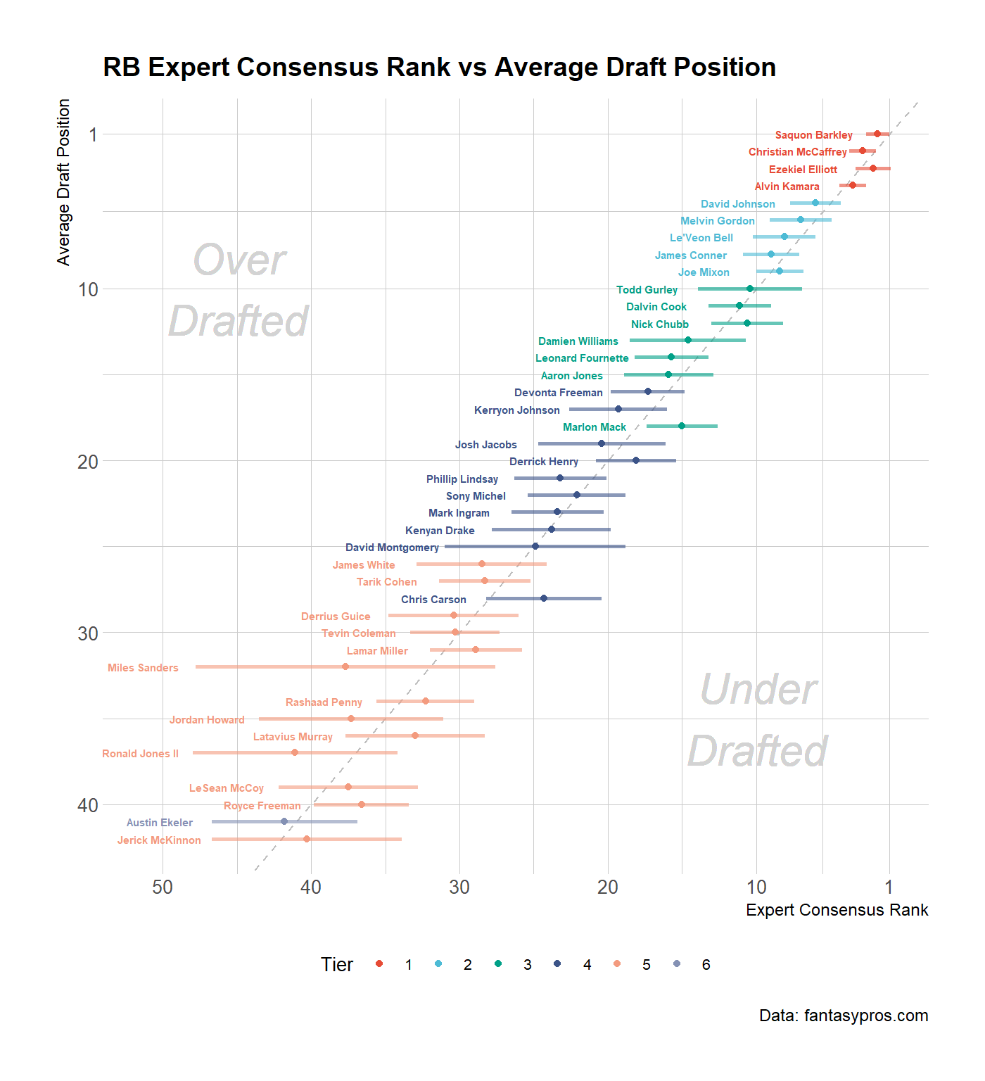
Visualizing Expert Consensus Ranking
library(fantasypros)
library(ggplot2)
library(dplyr)

fp_draft_rankings("RB") %>%
  filter(rank <= 40) %>%
  ggplot(
    aes(x = avg, y = adp, colour = factor(tier), label = player)
  ) +
  geom_abline(
    slop = 1,
    intercept = 0,
    linetype = 2,
    color = "grey"
  ) +
  geom_errorbarh(
    aes(xmin = avg - std_dev, xmax = avg + std_dev),
    height = 0,
    alpha = 0.6,
    size = 0.9,
    show.legend = FALSE
  ) +
  geom_point(size = 1.5) +
  scale_x_reverse(
    breaks = c(1, seq(10,70, 10))
  ) +
  scale_y_reverse(
    breaks = c(1, seq(10,60, 10))
  ) +
  ggsci::scale_color_npg() +
  hrbrthemes::theme_ipsum_rc(
    base_size = 10,
    axis_title_size = 9,
    plot_title_size = 14
  ) +
  labs(
    title   = "RB Expert Consensus Rank vs Average Draft Position",
    colour  = "Tier",
    x       = "Expert Consensus Rank",
    y       = "Average Draft Position",
    caption = "Data: fantasypros.com"
  ) +
  geom_text(
    aes(x = avg + std_dev),
    size = 2,
    nudge_x = -3.5,
    show.legend = FALSE,
    fontface = "bold"
  ) +
  geom_text(
    aes(x = 10, y = 35), label = "Under\nDrafted", color = "light grey",
    size = 8, family = "Roboto Condensed", fontface = "italic"
  ) +
  geom_text(
    aes(x = 45, y = 10), label = "Over\nDrafted", color = "light grey",
    size = 8, family = "Roboto Condensed", fontface = "italic"
  ) +
  theme(
    legend.position = "bottom",
  ) +
  guides(
    colour = guide_legend(nrow = 1)
  )
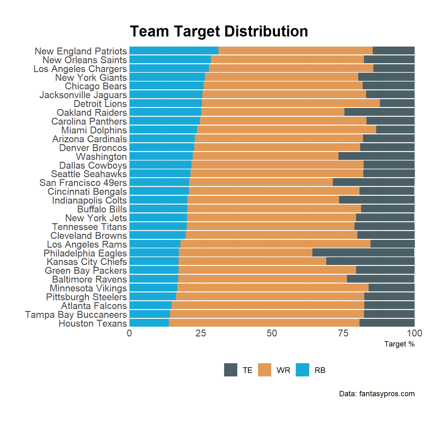
Team Target Distributions
library(fantasypros)
library(tidyverse)
library(ggplot2)

fp_team_targets(season = 2018) %>%
  select(
    team,
    ends_with("percent")
  ) %>%
  mutate(
    team = forcats::fct_reorder(team, rb_percent)
  ) %>%
  gather("position", "percent", -team) %>%
  mutate(
    pos = factor(
      position,
      levels = c("te_percent", "wr_percent", "rb_percent"),
      labels = c("TE", "WR", "RB")
      )
  ) %>%
  ggplot() +
  geom_col(
    aes(team, percent, fill = pos), alpha = 0.9
  ) +
  scale_x_discrete(expand = c(0, 0)) +
  scale_y_continuous(expand = c(0, 0)) +
  ggsci::scale_fill_jama() +
  hrbrthemes::theme_ipsum_rc() +
  coord_flip() +
  labs(
    title   = "Team Target Distribution",
    fill  = NULL,
    y       = "Target %",
    x       = NULL,
    caption = "Data: fantasypros.com"
  ) +
  theme(
    legend.position = "bottom"
  )
Season Stats
library(fantasypros)

fp_stats("QB", season = 2018, start_week = 3, end_week = 8)
#> # A tibble: 151 x 23
#>    player pos   team  season start_week end_week scoring passing_cmp
#>    <chr>  <chr> <chr>  <dbl>      <dbl>    <dbl> <chr>         <dbl>
#>  1 Aaron~ QB    GB      2018          3        8 half            124
#>  2 Alex ~ QB    WAS     2018          3        8 half             90
#>  3 Ben R~ QB    PIT     2018          3        8 half            132
#>  4 Brett~ QB    TEN     2018          3        8 half              0
#>  5 Brian~ QB    BUF     2018          3        8 half              0
#>  6 Brian~ QB    NE      2018          3        8 half              0
#>  7 Brock~ QB    DET     2018          3        8 half              0
#>  8 Byron~ QB    PIT     2018          3        8 half              0
#>  9 Chad ~ QB    KC      2018          3        8 half              0
#> 10 Chad ~ QB    MIA     2018          3        8 half              0
#> # ... with 141 more rows, and 15 more variables: passing_att <dbl>,
#> #   passing_pct <dbl>, passing_yds <dbl>, passing_y_a <dbl>,
#> #   passing_td <dbl>, passing_int <dbl>, passing_sacks <dbl>,
#> #   rushing_att <dbl>, rushing_yds <dbl>, rushing_td <dbl>, fl <dbl>,
#> #   g <dbl>, fpts <dbl>, fpts_g <dbl>, own <dbl>
Weekly Snap Counts
library(fantasypros)

fp_snap_counts(season = 2018)
#> # A tibble: 505 x 23
#>    player pos   team  season    w1    w2    w3    w4    w5    w6    w7
#>    <chr>  <chr> <chr>  <dbl> <dbl> <dbl> <dbl> <dbl> <dbl> <dbl> <dbl>
#>  1 Aaron~ QB    GB      2018    46    77    69    76    81    71    NA
#>  2 Adria~ RB    WAS     2018    42    25    32    NA    13    37    34
#>  3 Alex ~ QB    WAS     2018    79    74    61    NA    61    70    60
#>  4 Ben R~ QB    PIT     2018    84    82    66    62    60    73    NA
#>  5 Benja~ TE    NE      2018    51    54    45    37    36     0    36
#>  6 Brian~ QB    NE      2018     0     0     0     4     0     0     0
#>  7 Chad ~ QB    KC      2018     0     0     0     0     0     0     0
#>  8 Chase~ QB    CHI     2018     0     0     0     3    NA     0     1
#>  9 Danny~ WR    DET     2018    45    44    31    42    53    75    55
#> 10 Delan~ TE    TEN     2018    39     0     0     0     0     0     0
#> # ... with 495 more rows, and 12 more variables: w8 <dbl>, w9 <dbl>,
#> #   w10 <dbl>, w11 <dbl>, w12 <dbl>, w13 <dbl>, w14 <dbl>, w15 <dbl>,
#> #   w16 <dbl>, w17 <dbl>, ttl <dbl>, avg <dbl>

fp_snap_counts(pos = "defense", season = 2018, percentage = TRUE)
#> # A tibble: 769 x 23
#>    player pos   team  season    w1    w2    w3    w4    w5    w6    w7
#>    <chr>  <chr> <chr>  <dbl> <dbl> <dbl> <dbl> <dbl> <dbl> <dbl> <dbl>
#>  1 Patri~ CB    ARI     2018    99   100    99    98    97   100    98
#>  2 Adria~ DE    ATL     2018    30    30    42    37    51    33    40
#>  3 Princ~ CB    CHI     2018    98   100    50     0    NA    67    98
#>  4 Marce~ DT    JAC     2018    65    75    68    57    66    60    53
#>  5 Camer~ DE    PIT     2018    85    86    73    74    71    80    NA
#>  6 Von M~ LB    DEN     2018    88    77    68    68    74    70    85
#>  7 Rober~ DE    DAL     2018    59    51    71    56    68    71    58
#>  8 J.J. ~ DE    HOU     2018    93   100    84    87    90    87    90
#>  9 Justi~ DE    IND     2018    77    85    94    97    27     0     0
#> 10 Ryan ~ LB    WAS     2018    68    82    83    NA    73    80    74
#> # ... with 759 more rows, and 12 more variables: w8 <dbl>, w9 <dbl>,
#> #   w10 <dbl>, w11 <dbl>, w12 <dbl>, w13 <dbl>, w14 <dbl>, w15 <dbl>,
#> #   w16 <dbl>, w17 <dbl>, ttl <dbl>, avg <dbl>
Detailed Snap Analysis
library(fantasypros)

# all offensive positions for weeks 5-9 of the 2018 season
fp_snap_analysis(season = 2018, start_week = 5, end_week = 9)
#> # A tibble: 423 x 17
#>    player pos   team  season start_week end_week scoring games snaps
#>    <chr>  <chr> <chr>  <dbl>      <dbl>    <dbl> <chr>   <dbl> <dbl>
#>  1 Aaron~ QB    GB      2018          5        9 half        4   278
#>  2 Adria~ RB    WAS     2018          5        9 half        5   157
#>  3 Alex ~ QB    WAS     2018          5        9 half        5   328
#>  4 Ben R~ QB    PIT     2018          5        9 half        4   283
#>  5 Benja~ TE    NO      2018          5        9 half        4   119
#>  6 Brian~ QB    NE      2018          5        9 half        1     2
#>  7 Chase~ QB    CHI     2018          5        9 half        2     4
#>  8 Danny~ WR    MIA     2018          5        9 half        5   295
#>  9 DeSea~ WR    TB      2018          5        9 half        4   155
#> 10 Drew ~ QB    NO      2018          5        9 half        4   258
#> # ... with 413 more rows, and 8 more variables: snaps_gm <dbl>,
#> #   snap_percent <dbl>, rush_percent <dbl>, tgt_percent <dbl>,
#> #   touch_percent <dbl>, util_percent <dbl>, fantasy_pts <dbl>,
#> #   pts_100_snaps <dbl>
Weekly Targets
library(fantasypros)

# total targets for TE's in the 2014 season
fp_targets(pos = "TE", season = 2014)
#> # A tibble: 134 x 22
#>    player team  season    w1    w2    w3    w4    w5    w6    w7    w8
#>    <chr>  <chr>  <dbl> <dbl> <dbl> <dbl> <dbl> <dbl> <dbl> <dbl> <dbl>
#>  1 Zach ~ SEA     2014     4     1     2    NA    NA    NA    NA    NA
#>  2 Luke ~ SEA     2014     1     0     0    NA     4     6     0     4
#>  3 Andre~ GB      2014     4     2     5     0     2     5     1     3
#>  4 Ryan ~ CLE     2014     0     0     0     0     0     0     0     0
#>  5 Richa~ GB      2014     0     1     0     2     1     0     2     5
#>  6 Antho~ KC      2014     6     4     2     1     7    NA     1     4
#>  7 Travi~ KC      2014     5     6     4     9     3    NA     4     6
#>  8 Taylo~ TEN     2014     2     1     1     0     0     0     0     0
#>  9 Delan~ TEN     2014     4    14     7     7     4     8     5     9
#> 10 Beau ~ TEN     2014     0     0     0     0     0     0     0     0
#> # ... with 124 more rows, and 11 more variables: w9 <dbl>, w10 <dbl>,
#> #   w11 <dbl>, w12 <dbl>, w13 <dbl>, w14 <dbl>, w15 <dbl>, w16 <dbl>,
#> #   w17 <dbl>, ttl <dbl>, avg <dbl>